Solving Equations & Inequalities
Illustration 1. Here are some examples of quadratic
equations.
(a) The equation 3zx2−sx+4 = z is quadratic in x: a = 3z, b = −s
and c = 4− z. (Recall: We must write the equation in the form
3zx2− sx + (4 − z) = 0).)
(b) The equation 5wx4 −2w2x2+3 = 0 is quadratic in x2and also
quadratic in w.
(c) The equation 4 sin2(x)−4 sin(x)+1 = 0 is a quadratic equation
in the sin(x).
Comments: In example (b), the fact that the equation is quadratic
in x2means we can use the quadratic formula to solve for x2. The
same equation is quadratic in w means that we can use the quadratic
formula to solve for w. That’s the way it works!
Part of the power of the Quadratic Formula is that it is a very
efficient way of solving quadratic equations—more efficient than factoring,
usually—and it can be applied even when the coefficients a, b,
and c are symbolic. Here is a simple example.
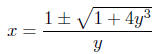
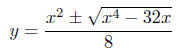
Illustration 2. Solve for x in the equation yx2
−2x−4y2= 0. This
is a quadratic equation in x because the highest power of x is power
2. We can applythe Quadratic Formula with a = y, b = −2 and
c = −4y2:
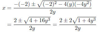
(In the last step, I’ve extracted 4 from the radical, which appears as
a 2 outside the radical.)
Note that we onlyget a solution when 1+4y3 ≥ 0. This
occurs when
 (Solving Inequalities is taken up
later.) (Solving Inequalities is taken up
later.)
Thus, for any y, 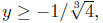 the solutions for x are the solutions for x are
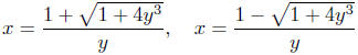
Exercise 7.10. The equation that appears in
Illustration 2 is a
quadratic equation in y. Use the Quadratic Formula to solve for
y.
Exercise 7.11. Use the Quadratic Formula to
(a) solve for w in
Illustration 1; and (b) solve for x2in the same equation.
7.3. Solving Inequalities
We encounter the problem of solving inequalities in a variety of settings.
For example, we stumbled across questions of solving inequalities
in the previous section on the Quadratic Formula. In that section,
our solutions came out in terms of symbolic quantities; recall the solution
to the equation discussed in Illustration 2:
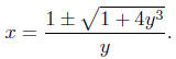
We only have “real solutions” (as opposed to solutions that are complex
numbers) provided
1 + 4y3 ≥ 0.
This is a (rather simple) problem of solving an
inequality
• Tools for Solving Inequalities
When you manipulate an inequality for the purpose of trying to isolate
the unknown on one side of the inequality, there are a few things you
should know.
Tools for Manipulating Inequalities:
a ≤ b =>a + c ≤ b + c (10)
a ≤ b and c >0 => ac ≤ bc (11)
a ≤ b and c <0 => ac ≥ bc (12)
a ≤ b and n ∈ N =>  (13) (13)
Tool Notes: Equation (10) states that you can add the same
quantity
to both sides of an inequality, and the inequality is preserved.
•By equation
(11), you can multiply both sides of an inequality
by a positive number and the inequality will be preserved.
•An
important variation on this is equation (12): If you multiply
both sides by a negative number the inequality is reversed. Caveat. It
is property (12) that most students have trouble with.
•Finally,
we can take a root of both sides and the inequality is
preserved. There is a built-in proviso: Provided the n^th roots of both
sides exist. This is not a problem when n is odd, but becomes one
when n is even.
Example 7.7. Let’s finish the analysis of
Illustration 2: In the
solution
we require 1 + 4y3 ≥ 0. Solve for y in this inequality.
• Simple Inequalities
The basic tools can be used to solve a simple class of inequalities:
Essentially Linear Inequalities.
Example 7.8. Solve each of the following
inequalities for x.
(a) 5x + 7 < 0 (b) 3 − 9x ≥ 4 (c) 3x5 + 4 ≥ 9 (d) 3x2 + 4 ≤ 3
Exercise 7.12. Solve each of the following inequalities for x. Write
your solutions in interval notation.

Here’s a slight variation on the previous problems.
Exercise 7.13. Solve each inequality for x. Leave your answer in set
notation.
(a) 2x − 1 ≤ 5x + 2 (b) 3x + 4 > 1 − 6x
• Double Inequalities
Bydouble inequalities I mean inequalities of the form
a ≤ b ≤ c (14)
as well as all variations on same. This notation is
short-hand for
a ≤ b and b ≤ c.
In this section we look at one simple type of problem—the case where
the b in (14) is a linear polynomial and a and b are constants.
This kind of problem can be solve in much the same way as in the
previous paragraphs.
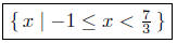
Illustration 3. Solve for x in −4 ≤ 3x − 1 < 6.
Solution:
| −4 ≤ 3x − 1 < 6 |
given |
| −4 + 1 ≤ 3x < 6 + 1 |
add 1 to all sides |
| −3 ≤ 3x < 7 |
combine |
| −1 ≤ x < 7/3 |
multiply all sides by 1/3 |
Presentation of Solution. Set Notation
Interval Notation: 
Illustration Notes: The standard tools for manipulating
inequalities
hold. You can add the same quantity to all sides of the inequalities
and you can multiply the same quantity to all sides.
•If you multiply all sides by a negative number, all the inequalities
are reversed!
Exercise 7.14. Solve each of the following for x.
Use interval notation
to express your answer. Passing is 100%.
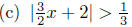
(a) 3 < 2x + 1 ≤ 12 (b) −2 ≤ 2 − 5x ≤ −1 (c) 1 < (3/2)x + 1 < 4
Quiz.
1. What is the solution set to the inequality1 ≤ x ≥ −1?
(a) [1,+∞) (b) [−1, 1] (c)
 (i.e., no solution) (i.e., no solution)
2. What is the solution to the inequality −1 ≥ x ≥ 1?
(a) [−1, 1] (b) [1,+∞) (c)
 (i.e., no solution) (i.e., no solution)
3. What is the solution to the inequality3 ≤ 2x − 1 ≤ 1?
(a) [1, 2] (b)
 (i.e., no solution) (i.e., no solution)
EndQuiz.
• The Method of Sign Charts
More complex inequalities require different methods. The Method of
Sign Charts is a general method of analyzing inequalities provided
you can factor the algebraic expressions. Let me illustrate this method
with an example.
Suppose you have an inequality of the form
R(x) ≥ 0
where R(x) is a rational expression. The idea is to
factor the expression
R(x) completely—both numerator and denominator—and analyze
the sign of each factor. The Sign Chart is just a graphical way
of storing all the information.
The next example is important because it delineates the
steps and the
reasoning that goes into the Sign Chart Method. Read this example
carefully.
Example 7.9. Solve the inequalities for x:
(a) x2− 3x + 2 ≥ 0 (b) x ≤ x2.
Exercise 7.15. Solve for x in each of the
following.
(a) x2− x − 2 ≤ 0 (b) x3 − 4x2+ 3x > 0
Tip. The basis for the Sign Chart Method is a comparison of some
algebraic expression with zero:
R(x) < 0 or R(x) > 0 or R(x) ≤ 0 or R(x) ≥ 0
Therefore, the first step is to put your inequality in one of the above
forms.
Exercise 7.16. Solve each of the following for x.
Write your answers
in interval notation.
(a) x2− 3x ≤ 4 (b) 6x −x2 < 5
This method is not limited to polynomial inequalities. The next example
illustrates the method for an inequality involving a rational
expression.
Example 7.10. Solve the inequality for 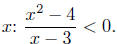
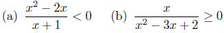
Exercise 7.17. Solve for x in each of the
following.
The Sign Chart Method is quite general and can be applied in a wide
variety of problems. To illustrate this statement, the next exercise continues
Exercise 7.10, which, in turn, was problem originally started
in Illustration 2.
Exercise 7.18. In order to have real solutions to
the equation in
Exercise 7.10, we require that the radicand in the solution
be nonnegative. Find all x for which x4 − 32x ≥ 0.
Let’s finish this section with a more challenging problem.
• Exercise 7.19. From Exercise 7.11, we used
the quadratic formula
to solve a fourth degree equation in x having symbolic coefficients in
terms of w. We obtained
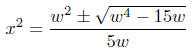 (15) (15)
In order for there to be real solutions (solutions belonging to the real
number system), we require (1) w4 −15w ≥ 0 and (2) the right-hand
side of (15) to be nonnegative. Your assignment, should you decide to
accept it, find all values of w that satisfy conditions (1) and (2).
7.4. Solving Absolute Inequalities
We finish this lesson by a short study of inequalities that involve the
absolute value function. We look at two type of inequalities:
|a| < b and |a| > b.
These two are a fundamental type in inequality that occurs rather
frequently in Calculus.
The method of solution is to (1) remove the absolute value
. . . in a
legal way; (2) solve the resultant inequality using standard techniques
described previously.
• Solving the Inequality |a| < b
The key to removing the absolute value from |a| < b is in the interpretation
of absolute value. Recall that
|a| = the distance a is from zero (0).
The inequality |a| < b then states that a is less than b units from the
origin. The fact that a is less than b units away from the origin would
be equivalent to saying that a is between −b and b. That is,
|a| < b is equivalent to − b < a < b
Let’s elevate this observation to the status of shadow box.
How to remove the | · | from |a| < b.
|a| < b <=> −b < a < b (16)
Note. Naturally, a similar statement is true for
|a| ≤ b; this is true if
and only if −b ≤ a ≤ b.
Once the absolute value is removed, we now have a double inequality—
which we solve.
Example 7.11. Solve each of the following for x.
(a) |x − 4| < 3 (b) |3x − 1| < 2 (c) |2 − 4x| ≤ 5
The method is simple enough, remove the absolute value, then solve
the double linear inequality.
Exercise 7.20. Solve each of the following for x.
Leave your answer
in interval notation. Passing is 100%.
(a) |x + 3| < 8 (b) |4x + 9| ≤ 1 (c) |2 − 7x| ≤ 3
• Solving the Inequality |a| > b
The solution to the inequality |a| > b can be concluded once the
absolute value as been removed.
A number a satisfies the inequality |a| > b if the distance it is away
from the origin is greater than b units. This means the value of a is
not in the interval [−b, b ] (for these are exactly the numbers that are
within b units of the origin). The number a we are looking for is not in
the interval [−b, b ]; therefore, the number a we seek must be greater
than b or less than −b. In symbols . . .
How to remove the | · | from |a| > b.
|a| > b <=> a > b or a < −b (17)
Note. A similar statement is true for |a| ≥ b: |a| ≥ b if and only if
a ≥ b or a ≤ −b.
The Split-Solve-Join Solution Method. The process of solving absolute
inequalities requires three steps.
1. Split: Split the absolute inequality using display line (17),
2. Solve: Solve the two inequalities, obtaining their solution sets.
3. Join: Join (take the union of) the solution sets from Step 2 to
obtain the final solution set to your absolute inequality.
Here are a couple of examples that illustrate the SSJS Method. Read
carefully.
Example 7.12. Solve each of the following for x.
(a) |x − 3| > 4 (b) |5x + 1| ≥ 3
Exercise 7.21. Using the SSJS Method, solve each of the absolute
inequalities for x. Write your answer in interval notation.
(a) |9x − 2| ≥ 3 (b) |2 − 3x| > 6
These same methods can be applied to more complicated absolute
inequalities. Here we have just considered absolute linear inequalities.
Equations and inequalities are the way w e can pose questions; therefore,
it is essential that we have very solid methods of solving equations
and inequalities. The techniques are demonstrated in this lesson are
far from being comprehensive, yet they will suffice you as you continue
to learn.
In the next lesson, we introduce the Cartesian Coordinate System
and discuss Functions. In Lesson 9 you will see how we use
equations and inequalities to pose questions; the techniques of this
lesson are then applied to solve.
Click here to continue to Lesson 8.
|